Area Estimation

Using image processing, we were taught to estimate an area desired using Green's Function. Green's function, as you know, relates a double integral to a line integral. This is very handy because by just traversing a line, we can be able to know the area enclosed by that line. Well, must have an enclosed line..

Numerically, the discreet form of the Green's theorem in obtaining the data, is like this:
where Nb is the number of pixels in the line or contour.

We first used different shapes. Shapes used were rectangle, triangle and a circle. We applied the Green's theorem in those shapes and then we compare the obtained area with the theoretical area.


Shape #1: Rectangle.

The rectangle used is a 400x400 pixel rectangle. Using the Green's function, it has obtained an area of 49170 pixels. Amazingly, the theorectical was 49170 pixels too. The picture and the code is shown below.

Figure 1: Rectangle

Result.



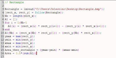Code for rectangle.

#note: If you notice, there is a line after the for loop that says A1(Nb). Because the limit of the for loop is until Nb-1, We have to show the value at Nb. Since we need the contour to be continous, Nb+1 = 1.
#note: Theoretical Area is obtained by finding the max and min of x and y, to find the length in pixels. Area is then a simple L x W.


For Triangle, the code is almost the same except for the theoretical area that is 0.5* B * H.

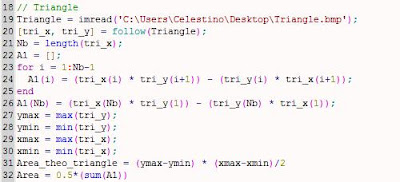
Code for Green's function in Triangle.

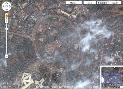
Image of the Quezon City Circle thanks to Google Maps. :)

First, aim is to obtain a black and white image of the contour of the QC circle like the previous shapes. What i did is that I highlighted the desired area white for i to have a constant value like this:

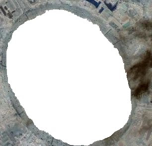
And then I used im2gray() and im2bw() to obtain a threshold for me to have a black and white image of the contour. It yielded this:

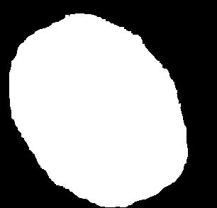
This is used in the Green's function program.

The code to obtain the Area using Green's function is shown below:



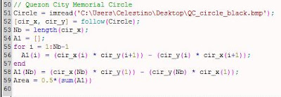
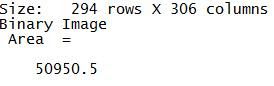
The Area obtained using this code is:

In order to get the Theoretical Area, I noted the coordinates of the end points of the two ds(D1 and d2). Since it is an ellipse, there is a need for two rs. (r1 and r2). By using the coordinates of the endpoints of the segments assumed as the diameter, the distance formula was used which obtained d1 = 287 and d2 = 213. Dividing them by half, we'll find r1 and r2 chich is 143.5 and 106.5 respectively. with this we can use the equation of an ellipse which is A = pi * r1*r2.
Theoretical Area yielded 47987.835 pixels. This is close to 50950 pixels. This is a 6% decviation from the theoretical. By the scale in google maps, it is found out that for every 200m, there is 87 pixel length. so, Total Area in meters will be 47987.835p * 200m/87p *200m/87p = 253121 square meters.

I think in this activity , I'd get an 9 out of 10. Because, I am able to do everything that is said. I got trouble checking the accuracy of my desired landmark due to software constraints.

It's Friday Blogging Night: Image formats

A couple of days ago, we were enlightened by the type of images we use and how these images are compressed and saved! And in this blog, I shall tell you what I have "seen". Apparently, those .png, .tif. .jpeg matters a lot when it comes to data storage specially if it involves images.

So what are these image types basically?

1. You know those black and white images? No? Yes? Well, they are called BINARY IMAGES. That's right! Binary like 1 and 0. because basically, the contents of those are *drumroll* 1 and 0. Yay! They are called BITS. And a 256x 256 image is only 8KB!An example of this is shown here:

This picture BITS really hard. Get it? *fake laugh* *embarrased*

note: this is only an example. file info of this is in indexed form. I can't find binary format.

2. Next on the list are GRAYSCALE images. If the binary was the cro-magnon, GRAYSCALE images are like the Cro-magnon .....with a CLUB. *dan dan dan* And a cro-magnon with a club is like more evolved. So why is it that it is called grayscale? Two words. Gray. Scale. Huh? Basically, It is like the binary but scaled in in 256 levels like in a Ragnarok Private Server. Information are recorded from 0 to 255 that's why there are a lot of shades of black that we say gray. A 256 x 256 grayscale image is around 64KB. Still don't know what a grayscale image is? See below:

Below.

note: the image is indexed. but for qualitative identification it it shown as grayscale.

3. This is when images discovered the Steam Engine! It gave color to the way we live. Next off are TRUEcolor images. And it does not LIE. Get it? No? Because it does not give FALSE information. Get it? No? Gaaaah. >__<. Truecolor images have channels or bands. These bands are usually in sets of 3. RGB. And the number of concentration of intensity in each band determines the color. These images are commonly seen in cameras. Specially, those cameras that take pictures of beauty.

This is Lena. Boys, behave! She's old. And this is a truecolor image of her.

FileName: C:\Users\Celestino\Pictures\Scilab pics\AP 186\trucolorimage.png
FileSize: 474648
Format: PNG
Width: 512
Height: 512
Depth: 8
StorageType: truecolor
NumberOfColors: 0
ResolutionUnit: centimeter
XResolution: 28.350000
YResolution: 28.350000

On a side note: A 256x256 true color image is around 192KB

4. Indexed image. This is when they junked the steam engine and became more efficient by making FORD motors to make gasoline engines. Instead of having 3 Bands of colors, They indexed color information on what they call a colormap. In this way, there are 2 sets of data being stored. This makes the image colored, and basically cover less memory space. Though it may reduce the color information.

Gaaawk! Polly wants an indexed cracker. Gaaawk!

FileName: C:\Users\Celestino\Pictures\Scilab pics\AP 186\Indexed image.png
FileSize: 25576
Format: PNG
Width: 150
Height: 200
Depth: 8
StorageType: indexed
NumberOfColors: 256
ResolutionUnit: centimeter
XResolution: 72.000000
YResolution: 72.000000

5. Other types. If number 4 is a gasoline engine. Next types are almost StarWars-y. They they are like the DeathStars because it is do high-tech. To mention a few, there are HDR in which recording are more than 8-bit. Multispectral and Hyperspectral where bands are not limited to RGB. And their name is so cooool. There are 3D images. They maybe the Chemical X in Imax-or not. They are used in MRI and CT(not City) scans. And lastly, the Cadillac of the movie industry, Temporal images or Video.

I didn't know Temporal Images makes me cry. Seriously.

Notice those file extensions like .jpeg .gif? These three little letters after the dot of your filemane matters. As you can see, these formats your image and then saves it. Here's the catch. In formatting, depending on the image format, there are some informations that are lost. Because in formatting, they are compressed to not allow hoarding of memory.

There are this lossLESS image compression in which EVERY PIXEL is PRESERVED. And the other is lossY image compression. Well, as the term implies it lossY-es information. What is the trade-off? The trade off is MEMORY. sweet sweet. MEMORY. That is why you need to know what type of file extension you need to use. If you need every bit for information, don't ya worry about saving memory. use .png, .tif extensions. if just for saving memory, use those lossY like .jpeg.

Results From The PRODECURE.

This is my initial scanned image:

What a graph.

It's size was 286 pixels for height and 320pixels for width. There is this 3 that I don't know what it says.

Taking Lena as my truecolor image, with its imfinfo up above, I tried to make a binary and grayscale image of her.

Lena again... Oh lala.

Grayscale image looked like this:

She's still beautiful aint she?

It has a size of 512 x 512

with imfinfo of:

FileName: C:\Users\Celestino\Pictures\Scilab pics\AP 186\trucolorimagegray.png
FileSize: 955736
Format: PNG
Width: 512
Height: 512
Depth: 16
StorageType: truecolor
NumberOfColors: 0
ResolutionUnit: centimeter
XResolution: 72.000000
YResolution: 72.000000

And this is when Lena is in Black and White:

Even in black and white, she dazzles me.

It has a size of 512x512.

And has a imfinfo of:

FileName: C:\Users\Celestino\Pictures\Scilab pics\AP 186\trucolorimagebw.png
FileSize: 21098
Format: PNG
Width: 512
Height: 512
Depth: 16
StorageType: truecolor
NumberOfColors: 0
ResolutionUnit: centimeter
XResolution: 72.000000
YResolution: 72.000000


Let us go back to the scanned image of the graph. This is a grayscaled image of the scanned graph.:

Grayscaled Gino004

And the Black and White image of the scanned graph after having to know the histogram of grayscale distribution, I used im2bw(, 0.9).

Black and White image.

As I can notice, the reconstructed Black and white image looked DARKER. It seems so because of the threshold value I put on the im2bw(). This somehow cleaned up certain colors.

By the way, little history on selected filename extensions on images.

1. JPEG
2. PNG


By the way, I think I'd have a grade of 8 out of 10 for this activity because I am unable to find certain types of images.


And I would like to acknowledge the help of my roomates. Wikipedia for certain images. Ang Maam Jing for most of the intellectual input.

Not so Scilab Basics

A while ago, we were given a somehow a crash course on Scilab. We used the 4.1.2 version because the toolbox that we are going to use somehow only works for the 4.++ versions.

Given the readings, I tried to familiarize myself to the instructions and syntaxes on Scilab. It looks very mush like python but with several differences.

At the end of the readings, we were given a set of exercises to do to make us refresh our programming skills and familiarize the programming language that is Scilab.

Initially, we were given an example on how to generate a centered circle. The code looks like this:

nx = 100; ny = 100; //defines the number of

elements along x and y

x = linspace(-1,1,nx); //defines the range

y = linspace(-1,1,ny);

[X,Y] = ndgrid(x,y); //creates two 2-D arrays of x

and y coordinates

r= sqrt(X.^2 + Y.^2); //note element-per-element

squaring of X and Y

A = zeros (nx,ny);

A (find(r<0.7)>

imshow (A, []);

where the words after "//" are comments. So that code basically generates an array that has a value of zeros per element then finds those indexes that satisfies r<0.7>

it looks like this:

Figure1. Circular Aperture

So we were asked to do different things.

We are to create synthetic images of:

a. centered square aperture

b. sinusoid along the x-direction (corrugated roof)

c. grating along the x-direction

d. annulus

e. circular aperture with graded transparency (gaussian transparency).

First off, I did the centered square aperture. It has this code:

// Square aperture

nx = 400; ny= 400;

x = linspace(-1,1,nx);

y = linspace(-1,1,ny);

[X,Y] = ndgrid(x,y);

A = zeros(nx,ny);

A(find(abs(X)<>

imshow(A, []);

And it gave the following image:

Figure 2. Square Aperture

I must say, this example taught me the powers of the '&' sign. :) I got stuck here because I always ended up making an off-axis square. Booo. But when I used the '&' sign, voila!

The corrugated roof generated this code:

// Sine

nx = 400; ny = 400;

x = linspace(-1,1,nx);

y = linspace(-1,1,ny);

[X,Y] = ndgrid(x,y);

A = sin(2*%pi*X.*5)

imwrite(A, 'C:\Users\Celestino\Pictures\Scilab pics\Sine.jpeg')

imshow(A, []);

And gave the following image:

Figure 3: Corrugated Roof

This figure showed the values of sin in the Y axis in terms of color. During the conception of the code, I got stuck because I dwelt in masking method that I forgot that it was simpler to plug in the equation of sine. Man, I really need to refresh my programming.

** Edit:

Sine fucntion have values ranging from -1 to 1. That's why there are little white lines in the images. Arvin Mabilangan told us that we have to set the range to be 0 to 1. So the edited code looks like this:

// Sine

nx = 400; ny = 400;

x = linspace(-1,1,nx);

y = linspace(-1,1,ny);

[X,Y] = ndgrid(x,y);

A = (sin(2*%pi*X.*5)+1)/2

imwrite(A, 'C:\Users\Celestino\Pictures\Scilab pics\Sine.jpeg')

imshow(A, []);

and yields this image:

Figure 3.5: Corrugated Roof version 2

Next up is the grating along the x-direction. It yielded this code:

// Grating

nx = 400; ny = 400;

x = linspace(-1,1,nx);

y = linspace(-1,1,ny);

[X,Y] = ndgrid(x,y);

a = sin(2*%pi*X.*5);

A = zeros(nx,ny);

A(find(a >= 0.1)) = 1

imwrite(A, 'C:\Users\Celestino\Pictures\Scilab pics\Grating.jpeg')

imshow(A, []);

And produced this image:

Figure 4: Grating

Nice thing about this code is that I used the previous corrugated roof and tweaked it a little to produce a grating. Basically, there is an array with zero value. What I did is that I set a threshold value for the sine function. This threshold if met will yield a value of 1. And that produced a grating.

The imshow function produces a non-uniform grating though when imwrite-ed, it gives a better and more accurate picture of the grating.

The annulus was coded like this:

nx = 400; ny = 400; // defines the number of elements along x and y

x = linspace(-1, 1, nx); // defines the range

y = linspace(-1, 1, ny);

[X, Y] = ndgrid(x,y); //creates a 2D array of x and y coordinates

r = sqrt(X.^2 + Y.^2); // note element per element squaring of X and Y

A = ones(nx,ny);

A(find(r<1))>

A(find(r<0.5))>

imwrite(A, 'C:\Users\Celestino\Pictures\Scilab pics\Annulus.jpeg')

imshow (A, []);

With an image that looks like this:

Figure 5: Annulus

This is relatively the easiest of the exercises given. Here, what I did is to tweak the example given to produce another circular aperture. After that, it is just a matter of adjusting the values necessary.

Lastly, for the circular aperture with graded transparency (gaussian transparency), I have made the code to be like this:

//Circular Aperture with graded transparency

nx = 400; ny = 400;

x = linspace(-1, 1, nx);

y = linspace(-1, 1, ny);

[X, Y] = ndgrid(x,y);

r = sqrt(X.^2 + Y.^2);

A = ones(nx,ny);

lambda = 10

A = exp(-(r)^2/lambda^2)

A(find(r<0.1))>

//A(find(r>0.25)) =exp(-(r.)^2/lambda^2

//A(find(r>0.25)) = 0

imwrite(A, 'C:\Users\Celestino\Pictures\Scilab pics\Gaussian2.jpeg')

imshow (A, []);

And yielded this image:

Figure 6: Circular Aperture with graded transparency

This one is hard. And I am not pretty sure I got this one right. What I did is to show a Gaussian circular decay and then masked a circular aperture. Adjustment for the desired image parameter is a lot of trial and error and the imshow does not help that much for giving an inaccurate image.

In this activity, I think I'll grade myself 8 out of 10. Because Gaaah! I suck at programing. And I don't know if I got the graded transparency right.

I'd like to thank Andy Polinar, Arvin Mabilangan, Gino Leynes and Maam Jing Soriano for helping me figure out how to code these exercises in Scilab.

Thanks for reading. Comment if there are any mistakes.

First AP186 Activity

In this first activity, we were asked to obtain numerical values of a graph that is manually drawn. For us to do this, we are to use the scanned image of the graph and use its pixel location to be able to find functions that will able to relate the said pixel location to the true value in the graph.

The hand-drawn graph that I chose to reconstruct is a graph that shows a relation foreign salt concentration versus pH of ZnSO4 as shown in the succeeding picture.

Figure 1: Scanned image of a handmade graph.

Maxima and minima pixel location were determined using Paint program. By obtaining these locations, proper scaling methods can be used.

Let us first look at the Y-axis. This axis is pretty much simpler than the X-axis to scale for it explicitly tells us that it has a linear relation. It can simply be related as a starting Y intercept with a value of 3.5pH and as pixels move closer to the top pixel, it linearly approach the value of 6.0pH.

Scaling factor is found by looking at the Y-pixel location of 4.5pH which is 384. As seen, a 1 pH change results to a change of 237 pixel.

The final scaling formula for the pixel to pH relation is:

3.5pH + (no. of pixel * 1pH/237 pixel) = pH

Further modification is that since Paint counts Y pixels from top to bottom(normally it's bottom to top) no. of pixel is modified as:

no. of pixel final = 621- no of pixel

This modification errors of about 15 pixels for I was unable to extract the exact value though this modification is a near approximation on the reconstructed image.

Looking at the X-axis, it can be seen that it is not linear. Scaling formula is that it is exponential that looks like this:

Concentration of foreign salt = (M/4096) * (2^N)

where N is the linear factor of the function.

N here is dependent on the X-axis pixel location of the graph. The total pixel area to be considered in scaling N is equal to 644 pixel- this was from 132 to 776 pixel maxima and minima. There were 12 division considered so N can be obtained as:

N = (12/644 pixel) * (pixel location)

By establishing these relations, I can simply plug-in the coordinates of the X and Y pixels and the natural value can be obtained. This is where Microsoft Excel and Office Office Spreadsheets comes in handy. I plugged in the relations and the coordinates and was able to obtain values. Sample calculations are shown below:

Figure 2: Sample Calculations of Natural values from Scanned Graph

Graph was fitted in terms of N for it is the linear scale for the graph. If it be the natural value of the Concentration, graph may have the same form but will have wider and more compact sections of the graph.

Fitted and overlayed graphs are shown here:

Figure 3: Fitted and overlayed graph of the scanned and the reconstructed.

It can be seen that the reconstructed part considered was from the M/4096 to M/4. It is because I am unable to relate M/4096 to 0 generally with the M/4096 to M/4.

I'd say I think out of 10, I'd grade myself 10 for I was able to reconstruct the image using the methodologies and utilities needed.

I'd like to thank Maam Jing for helping me with scaling the x axis, Aivin for helping me figure out Open Office because there was a time a while ago that I was really freaking out because I can't format the spreadsheet's cells and Jane for lending me her laptop for my laptop is crappy and broken.

Thanks for reading. This is one of the times that I will post seriously. LOL